This comprehensive exploration of acoustic engineering covers the fundamental principles behind ultrasound medical imaging. The work represents a sequential building upon key topics in acoustics, from beam focusing to signal processing, all with direct applications to the technology that provides windows into the human body.
This topic is near and dear to me as it heavily overlaps with my professional life. The methodology and results of each major topic are self-contained and represent real applications of the science behind medical ultrasound technology.
Beam Focusing with Rayleigh Sommerfeld Method
Methodology and Results
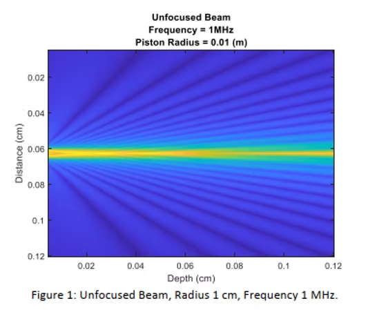
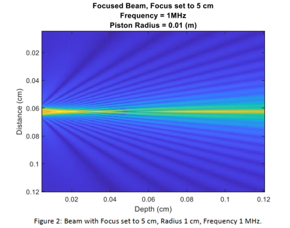
The first challenge was taking an unfocused beam and using the numerical Rayleigh Sommerfeld method to focus it. This classic circular piston problem used a specified radius of 1 cm, mimicking a cardiac phased array probe. The objective was to plot the continuous wave beam at 1 MHz out to 12 cm in water, then repeat the exercise for a focus at 5 cm.
Key Insight
With deep gratitude, the partial solution was shown in concept without giving away the implementation details. The solution relied on 9th grade geometry principles applied to complex acoustic wave propagation.
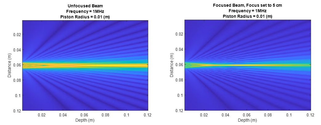
Here are the initial results before optimization. The unfocused beam is on the left and the focused beam is on the right:
Initial attempts - the results didn't feel good and looked about as good as they felt
The initial results were problematic - the axis labels were wrong and the focusing wasn't working properly. After coffee and more careful MATLAB work, the results improved significantly:
Improved results showing clear beam convergence at 0.04 m - much better!
This problem was particularly satisfying because the results are quite visible. A clear convergence can be seen at 0.04 m, demonstrating the effectiveness of the Rayleigh Sommerfeld numerical method for beam focusing calculations.
Complex Analytic Signal Processing
Methodology
The next challenge involved finding the magnitude of the complex analytic signal from both simulated and real RF waveforms (A-scan, one dimensional). The process involved several key steps using MATLAB:
Signal Processing Steps:
• Find the FFT of the signal
• Zero FFT bits to produce the spectrum of analytic signal, using frequency cutoff to eliminate frequencies outside the passband
• Compute the IFFT of the analytic spectrum and double it to produce the complex analytic signal
• Take the magnitude of the complex analytic signal
• Plot the signal and the magnitude of the complex analytic signal together
Results
The simulated and measured signals with their extracted envelopes:
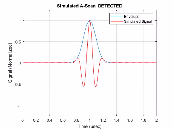
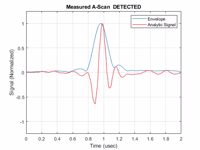
Simulated (left) and measured (right) RF signals with extracted envelopes
The original signal processing challenge:
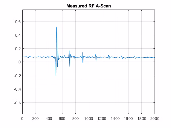
Original RF waveform used for envelope extraction
Bonus Challenge: Built-in MATLAB Function
Using MATLAB's built-in 'envelope' function proved surprisingly effective, getting very close to the manual implementation results with numerous options for fine-tuning.
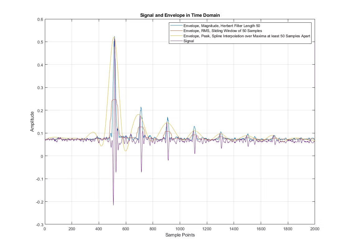
Results using MATLAB's built-in envelope function - impressively close to manual implementation
Double Bonus: Custom Filter Approach
Low-pass Chebyshev2 and Butterworth filters were also tested for envelope detection. Results were less predictable, with filter parameters having significant impact on effectiveness. The filters followed the original signal peaks too closely, requiring more refinement.
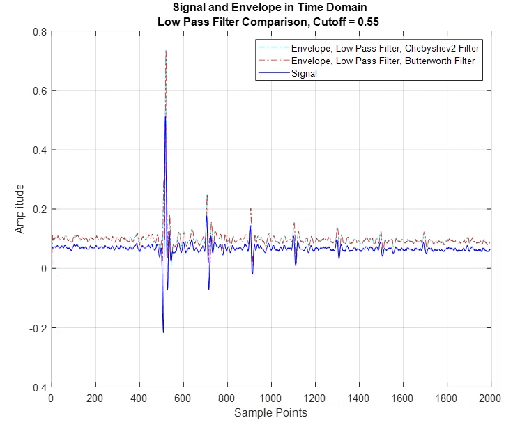
Custom filter results - following peaks too closely, more work needed for optimal performance
Resolution Enhancement
Challenge
Given a pulse echo signal, the goal was to shorten the transmitted pulse length to achieve improved resolution, then determine what else could be changed without modifying the transducer to achieve a 2x improvement in resolution.
Results
The image below shows a summary of adjustments made to achieve optimum resolution. Note the progression from fuzzy, thick white bars to much cleaner, well-defined features:
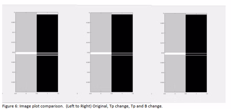
Resolution improvement progression: original (left), halved pulse length (center), optimized bandwidth (right)
The left image shows the original pulse echo signal with characteristic fuzzy white bars across the middle. The center image was created with a halved transmit pulse length. The reason a full 2x improvement isn't seen is because only the transmit electrical pulse length was adjusted - this is only part of the resolution battle.
The other major component is transducer bandwidth. When this is adjusted along with the halved electrical pulse, we achieve much closer to a 2x improvement in resolution. This can be practically achieved by adjusting the bandpass filter range to allow more signal through, though there are practical limits.
Frequency Impact
For the final part, transmit frequency increased from 5 MHz to 10 MHz. This seemingly simple change dramatically reframes the design problem:
5 MHz crystal thickness: 0.154 mm
10 MHz crystal thickness: 0.077 mm
This significant reduction impacts manufacturing cost, expertise requirements, breakage rates, and ultimately transducer pricing.
Delay and Sum Beamforming
Concept
Echoes and their reflections, when delayed to be made "flat," then summed to show overall brightness level using the magnitude of the Hilbert transform, create an image! This is the fundamental principle behind ultrasound imaging.
Process and Results
Starting with echoes from targets at 1 and 2 cm respectively, the process involves time-aligning (flattening) the signals:
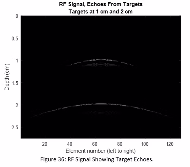

Original echoes from targets (left) and the time-aligned "flattened" versions (right)
The final step applies the magnitude of the Hilbert transform after summing all the aligned signals:
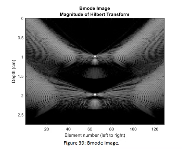
Final beamformed image showing the targets as bright spots
Contrast Analysis
Overview
Contrast is a rich subject with extensive applications in ultrasound imaging. At its core, contrast involves comparing adjacent regions' average peak values. While Speckle SNR, envelope variance, and envelope mean are all important parameters, the fundamental concept is the comparison of adjacent regions.
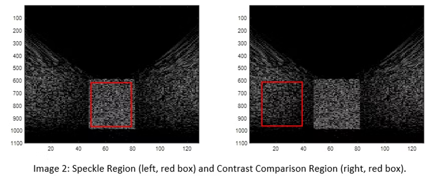
Speckle region (left) and contrast region (right) used for contrast calculations
To calculate Contrast for this image, we use: 20*log10(SpeckleMean/ContrastMean). Depending on the context, these regions may be swapped, but the calculated value provides the important quantitative measure of image contrast quality.
Personal Reflection
This comprehensive journey through acoustic engineering provided deep insights into how ultrasound technology actually works. Learning how basic concepts are calculated and discovering new mathematical applications was incredibly rewarding. The work gave me tremendous appreciation for the colleagues I work with and their ability to transform these concepts into medical technology that helps people.
I'll never forget the times my wife was pregnant with each daughter, and how fortunate we were to have medical care that provided a window into our future through ultrasound. The technology that seemed so magical then now has concrete mathematical foundations that I can understand and appreciate on a much deeper level.
Key Learning Outcomes
• Understanding the mathematical foundations of medical ultrasound
• Hands-on experience with beam focusing and signal processing
• Appreciation for the engineering challenges in medical device development
• Connection between academic theory and real-world medical applications
This work represents not just academic exercises, but real understanding of technology that touches millions of lives. The intersection of physics, mathematics, and medicine creates truly inspiring applications of engineering knowledge.