Wireless Communication Projects

Project 1: Receiver Performance in Noise & Fading Channels

Setup

Methodology

Assuming coherent detection and perfect estimation by the receiver, the following equations for BPSK, QPSK, and DBPSK were used to predict theoretical performance:

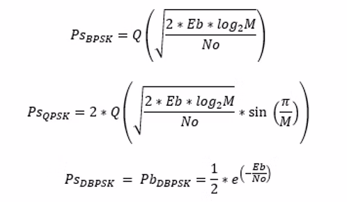
Theoretical performance equations for BPSK, QPSK, and DBPSK modulation schemes

For a binary scheme, Eb = Es and the formula for symbol error probability and bit error probability are equal. Signals were randomly generated for BPSK as ±1. QPSK signals were randomly generated as ±1±j, and DBPSK signals were randomly generated as 0 or 1. Noise was then generated by determining the square root of the variance σ, for each scheme, as shown below:

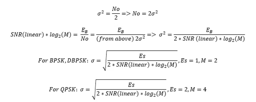
SNR calculations and noise variance relationships for simulation

Sigma was then multiplied by real Gaussian noise. Complex noise was generated for QPSK and DBPSK (non-complex noise was generated for BPSK). Signals were combined and the thresholds were determined based on potential outcomes. For the two BPSK schemes, the received signal was compared element-wise to the generated signal and any time they were not equal, it was counted as an error. Similarly for QPSK, the real and imaginary parts of the signals were compared element-wise to the generated signal and inequalities were counted as errors. The error counts were then used to determine SER.

For DBPSK, the original signal of 0 or 1 was first differentially encoded. Zeros were then changed to ±1 before complex noise was added, then the comparison to the original signal was performed with the threshold to determine SER. Also unique to DBPSK, the complex conjugate of the detector input was taken with the prior value to determine the comparator signal. This was done with the intention of representing the structure of a DBPSK receiver that compares the received value with its predecessor to determine whether a difference was transmitted.

Rayleigh Fading Channel

To address the second problem, the following equation was used to model Rayleigh fading:

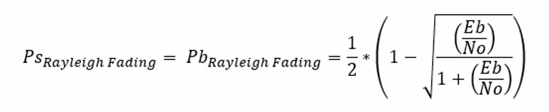
Rayleigh fading channel model equations

To address the last problem, the sum of sinusoids method was used:

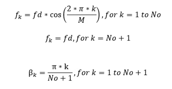
Jake's model parameters for channel simulation

For the fading channel, the real and imaginary components were found using the following equations:

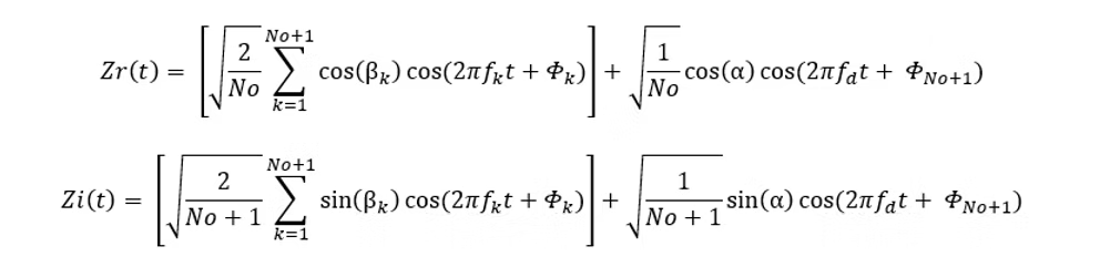
Real and imaginary components of the fading channel model

Results

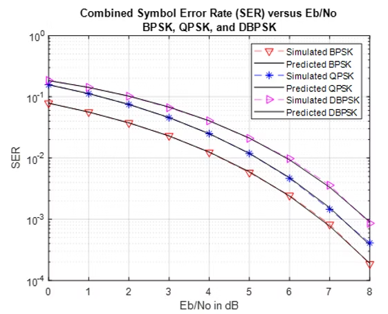
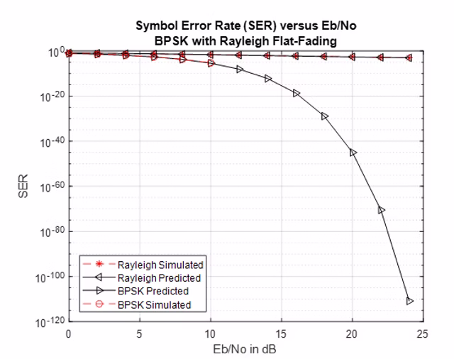
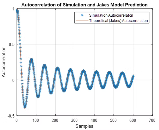
The left image below shows the SER (theory versus simulated) for BPSK, QPSK, and DBPSK. The center image below shows the SER (theory versus simulated) for a Rayleigh flat-fading channel (compared to BPSK for reference). The right image below shows the autocorrelation of the Jake's Model prediction and the simulation:

Performance results: SER comparison, Rayleigh fading effects, and Jake's model validation

In all of the cases, the simulated versus theoretical plots align fairly well. For the SER plot on the left (above), the sample rate has a significant impact on performance - decreasing the number of samples worsens performance as SNR is increased. The SER plot of the Rayleigh flat-fading channel shows the true meaning of "flat-fading" - the SER as SNR is increased is nearly unchanged compared to BPSK. Finally, the plot on the right (above) shows that the correlation of model versus prediction aligns very well, and is ultimately very similar to a Bessel function.

In all, this was a great exercise to map the received signal under basic conditions. Generally, as SNR increases, the error rate decreases for the schemes tested here. In the real world however, many more conditions require accounting for under different receive schemes (64-QAM, for example).

This project taught me so much about signal reception, channel modeling, and performance as well as new ways to utilize the power of Matlab.

Project 2: Transmit & Receive Diversity Systems

Setup

In the second project, I explored two types of diversity - Receive and Transmit. These again were compared, pitting simulation versus model predictions using signals generated from Matlab. BPSK and QPSK modulation was used and receive diversity was evaluated using Selection Combining, Maximal Ratio Combining, and Equal Gain Combining. Transmit diversity was evaluated using Maximal Ratio Transmission and the Alamouti space-time coding scheme.

Methodology

Assuming again coherent detection with perfect receiver estimation, we add to the list of assumptions: 1. the average power of the channel gain is equal to 1, and 2. the SER performance of the receivers would be conducted by simulating samples at the output of the correlator receiver, with bit energy equal to 1.

Signals and noise were generated in the same way as presented in the first project (including variance) and won't be duplicated here.

The vector of the complex channel gain of each independent path over Rayleigh fading was modeled as shown in the first equation below, followed by the general model equation:

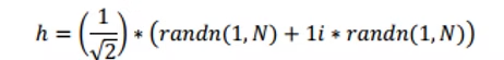
Channel modeling equations for diversity system analysis

Receive Diversity Techniques

Selection Combining (SC) receiver diversity selects the received channel with the highest SNR and runs with it. This means that no channel information is needed for this method. For a single channel, the SER is quite similar to a Rayleigh fading channel but for more than one channel, the SNR was calculated to find the highest value before determining the Bit Error Rate. Given the assumptions stated above, plus the noise being zero-mean and Gaussian distributed, the noise was assumed to be relatively equal for all branches. For SC, we simply pick the highest SNR.

Maximal Ratio Combining (MRC) creates a combined weighted sum of each branch for each number of antennas. As this requires knowledge of the channel at the receiver, it's a bit more complicated. Each branch is weighted with the conjugate of the complex gain of each branch. The applied weight was determined through instantaneous SNR analysis. The Cauchy-Schwarz inequality was used to find that the SNR is maximum when wH = hH. We then co-phase the signals by taking the conjugate of the channel gain as the weight and combining the signals together. This sum maximizes SNR.

Equal Gain Combining (EGC) receive diversity is different from MRC in that it does not estimate the SNR for each received signal. Instead, EGC co-phases each branch, then combines branches with unity gain.

Transmit Diversity Techniques

Maximal Ratio Transmission (MRT) takes advantage of knowledge of the channel at the transmitter. The signal is multiplied by the square root of the summed magnitude of each channel gain, then squared. Normalization is required to ensure the power transmitted is divided equally. Sort of like making sure that each teen-ager gets the same amount of stuff (M&Ms, popcorn, t-shirts, rides, etc. etc. etc.). MRT theoretical performance is modelled by using MRC because of the channel knowledge known early on.

Alamouti Space-Time Coding: For Alamouti, the channel is unknown at the transmitter. One way to achieve transmit diversity is to utilize Alamouti space-time coding. This coding transmits a combination of the first and second signal over two time periods, with the assumption that the channel is constant over the time periods. When the transmission is received, the receiver forms a vector with the two signals. The receiver multiplies the combined signal with a matrix, resulting in a decoupling of the two symbol transmissions. The final form is as follows:

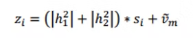
Alamouti space-time coding decoupling equations

There is a penalty of 3 dB to pay due to the receive SNR being equal to the total SNR from each branch, divided by 2.

Results

For brevity, the plot below shows the simulated versus theoretical performance for BPSK modulation receive diversity using SC, MRC, and EGC on the left. On the right, simulated versus theoretical performance for BPSK modulation using transmit diversity (MRT and Alamouti coding) is shown.

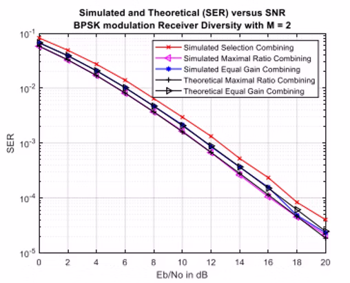
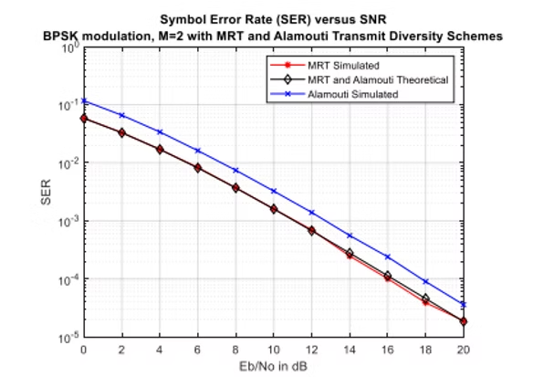
Diversity system performance: Receive diversity (left) and transmit diversity (right)

These plots (in combination with the individual performance plots) show that transmit and receive diversity methods are employed to lower the probability of deep fading on channels simultaneously when a signal is received. This means that reliability can be improved and "good" performance can be achieved with the proper technique (in terms of SER) on the transmit and receive sides.

If the channel information is unknown, Alamouti space-time coding performs within 3 dB of MRT, allowing for a simple and clever way to realize good performance.

Reflection

My biggest takeaway from these projects is the appreciation of projects like the Voyager space program and others that had to have an answer for reliable transmission of information across large distances. These concepts have been around for a long time and I am in total awe...

My growing interest in this field has led to some Software Defined Radio projects, which I'll add to the site in the future.